Instructions
Worksheets
Overview
The goal of this week’s experiment is to first characterize a spring by measuring its spring constant, and then measure the behavior of the spring when it is hung vertically with a mass on one end and allowed to oscillate. The period of oscillation, or the time required for the spring to complete one cycle of its motion, will be measured experimentally, predicted using a theoretical model, and calculated using a VPython simulation.
Experimental Measurements
 |
 |
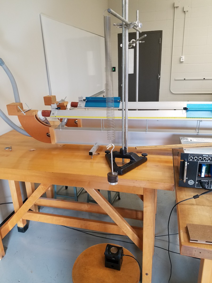 |
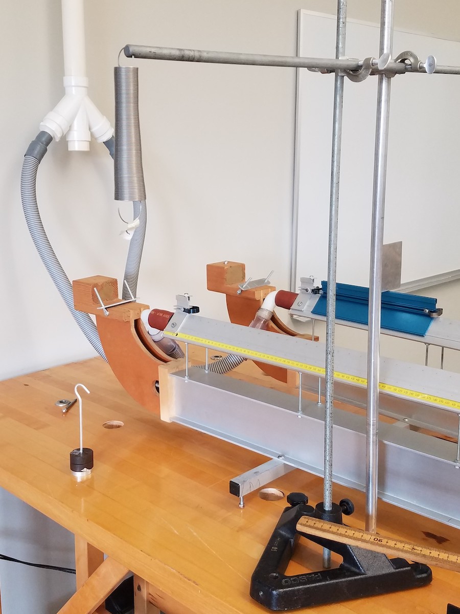
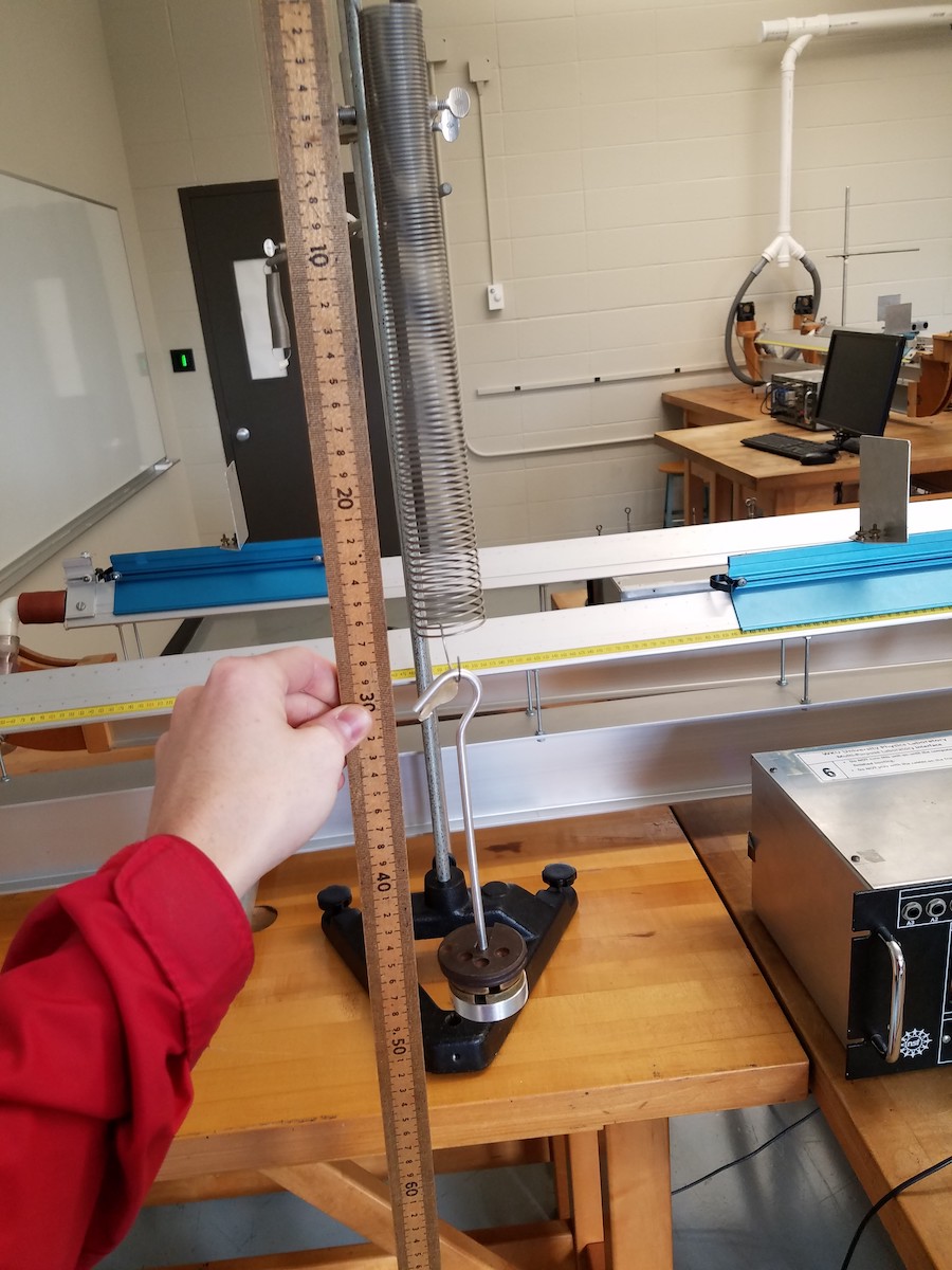
| Figure 1: Vertical Spring | Figure 2: Measuring Stretch | Figure 3: Measuring Oscillation |
A conical spring of mass 0.0915 kg was hung vertically from a pole as shown in Figure 1. Masses were attached to the bottom of the spring and the position of the mass relative to the top of the spring was measured as shown in Figure 2. Results for 5 different masses are shown in the table below.
| Mass kg |
Force N |
Position ± 0.005 m |
| 0.25 | 0.480 | |
| 0.30 | 0.525 | |
| 0.35 | 0.570 | |
| 0.40 | 0.610 | |
| 0.55 | 0.730 |
These data will allow you to determine the spring constant of the spring. After doing so, use your results to predict the position when a 0.45 kg mass is attached to the spring. Compare your predicted position for this 0.45 kg mass to the measured value of 0.655 m.
After setting the spring into oscillation, the position of the mass was measured using the sonic ranger. The following file contains the position versus time as the 0.45 kg mass oscillated on the spring.
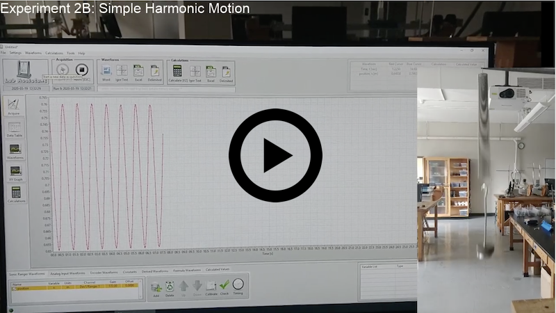
Video
The video below shows an example of data being collected in the Physics Lab Assistant software while the mass on the end of the spring is oscillating. The synchronization between the inset and the software isn’t perfect but it gives a great overview of how the data is acquired.
Simulation
You will model the motion of a mass oscillating on a vertical spring.

Begin by copying and pasting the starter code in the box below into a new GlowScript program. This code will draw a rectangular box named ceiling to simulate the ceiling or other structure to which the spring is attached, and a helix named spring to simulate the spring, and a small cylinder named hanger to simulate the hanging mass. Initially the system will be displayed stationary. You will make changes (described below in steps A thru D) that will realistically simulate the motion of the mass as it oscillates up and down on the spring.
The code has built in options to be able to display the unloaded (no mass) spring at its natural length along with another image that will show the spring with the mass hanging in equilibrium. These images can be useful to get a better understanding of how the mass will oscillate on the spring. These options can be enabled or disabled by setting the boolean flags named showUnloaded and showEquilibrium to True or False respectively. The unloaded spring will appear to the left and the spring-mass system in equilibrium will appear to the right of the simulated spring system.
Additional information about how to compute the force exerted on the mass by the spring can be found in the tutorial Modeling a Spring Using Hooke’s Law.
A – Enter Constants to Describe the System
In the appropriate variables enter the names of the students in your group, and the requested characteristics of the spring and the mass hanger.
B – Enter Initial Conditions for the Mass Hanger
The coordinate system that is used has the \(y\)-axis in the vertical direction with positive\(y\) upward and negative\(y\) downward as usual. The origin of the coordinate system is at the point where the spring is attached to the support “ceiling”.
When the mass is hanging in equilibrium then the net force on the mass will be zero and we can find the amount the spring will be stretched using: $$F_{\textrm{net,y}} = 0$$ $$k_s s_0 – m g = 0$$ $$s_0 = \frac{mg}{k_s}$$
The spring, when hanging in equilibrium, will have a total length of \(L_0 + s_0\) and will have a y-coordinate of \(y_0 = -L_0 – s_0\). For convenience, the program defines a variable named y0 that equals the equilibrium position of the spring. You can enter initial positions relative to this equilibrium position as is shown in the starter code where the mass has been pulled down 10 cm below equilibrium (i.e. y0 - 0.10).
C – Enter All Forces Acting on the Mass and Find the Net Force
Enter appropriate vector expressions for the forces acting on the mass (gravity and spring force) and then compute the net force on the mass.
D – Update the Momentum and Position of the Hanger
Enter appropriate equations to update the momentum (hanger.p) and position (hanger.pos) of the mass hanger.
At this point your program should display the motion of a mass hanger on a vertical spring in the approximation of a massless spring and no air resistance.
#
# Motion of a Mass on a Vertical Spring
#

#############################################################################
#                                                                           #
# A - Enter student names and additional constant values for the system.    #
#                                                                           #
#############################################################################
students = 'Sally Smith and Johnny Jones'
L0 = 0.25                       # Natural (unstretched) length of spring (m)
rs = 0.02                       # Radius of the spring (m)
k  = 8.0                        # Spring constant (N/m)
m  = 0.15                       # Mass of hanger (kg)
rm = 0.04                       # Radius of the mass hanger (m)

# Additional constants
g  = 9.8                        # Acceleration due to Gravity (N/kg)
t  = 0                          # Time counter (sec)
dt = 0.01                       # Time step (sec)

# Compute some useful position values
s0 = m*g/k                      # Absolute value of the stretch of spring at equilibrium
y0 = -L0 - s0                   # y-coordinate when system is in equilibrium

# Flags to Show (True) or Hide (False) various aspects of than animation or graph output
showUnloaded = True        # Shows or hides an unloaded spring in the animation
showEquilibrium = True     # Shows or hides a stationary spring in equilibrium in the animation

# Set up the scene as a skinny vertical canvas on the left leaving room
# on the right for graphs.
scene.width  = 300
scene.height = 600
scene.center = vector(0, -L0, 0)
scene.align = "left"
scene.background = color.gray(0.7)

# Draw the supporting ceiling, placing the origin at the point of attachment of the spring.
ceiling = box(pos=vector(0,0,0), size=vector(1.5*L0, 0.01, 0.5*L0), color=color.black)

# Create an object for the mass hanger.
hanger = cylinder(color=color.red)

# Define additional attributes of the mass hanger.
hanger.radius = rm                          # Radius of the mass hanger (m)
hanger.m = m                                # Mass of the block (kg)
hanger.axis = vector(0, -0.01, 0)           # Set the height of the hanger to 1 cm.

#############################################################################
#                                                                           #
# B - Enter the initial position and initial velocity of the mass hanger.   #
#                                                                           #
# The mass will be in equilibrium when the length of the spring is L0 + s0, #
# which would correspond to a y-coordinate of y0 = -L0 - s0.  If you pull   #
# the mass down an extra 10 cm from this equilibrium position the initial   #
# position should be -L0 - s0 - 0.10 or y0 - 0.10.                          #
#                                                                           #
#############################################################################
hanger.pos = vector(0,y0-0.10,0)            # Initial position of the mass (m)
hanger.v = vector(0,0,0)                    # Initial velocity of the mass (m/s)
hanger.p = hanger.m * hanger.v              # Initial momentum of the mass (kg m/s)

# Draw the spring with one end attached to the ceiling and with a length equal
# to the initial position of the mass hanger.
spring =  helix(pos=vector(0,0,0), axis=hanger.pos, radius=rs,
                coils=15, thickness=0.004, color=color.gray(0.5))

# Show the unloaded (no mass) spring on the left if requested to do so
if (showUnloaded):
    helix(pos=vector(-L0/2,0,0), axis=vector(0,-L0, 0), radius=rs, coils=15, thickness=0.004, color=color.gray(0.5))
    text(pos=vector(-L0/2,L0/5, 0), text="UNLOADED", axis=vector(0, 1, 0), height=0.05*L0)

# Show the loaded spring hanging in equilibrium on the right if requested to do so.
if (showEquilibrium):
    helix(pos=vector(+L0/2,0,0), axis=vector(0,-L0-s0, 0), radius=rs, coils=15, thickness=0.004, color=color.gray(0.5))
    cylinder(color=color.red, axis = vector(0, -0.01, 0), radius = rm, pos=vector(L0/2,-L0-s0,0))
    text(pos=vector(L0/2,L0/5,0), text="EQUILIBRIUM", axis=vector(0,1,0), height=0.05*L0)

# Set up the graph of Position versus Time
graphTitle = 'Mass Spring System: ' + students + ', m = ' + hanger.m + ' kg, k = ' + k + ' N/m'
graph(title = graphTitle, width = 800, height = 400,
        xtitle = 'Time (s)', ytitle = "Displacement from Equilibrium, y-y0 [m]",
        fast = False, align="right")

PositionVsTime = gcurve(color = color.blue,  width = 2)

while (t<10):
    rate(100)

    # Compute the position of the mass relative to the attached end of the spring
    L = hanger.pos - spring.pos         # This is a vector !!
    spring.axis = L                     # Draw the spring the proper length

    #########################################################################
    #                                                                       #
    # C - Compute the forces exerted on the hanger by the spring and by     #
    # gravity.  Then compute the NET force.                                 #
    #                                                                       #
    #########################################################################


    #########################################################################
    #                                                                       #
    # D - Update the momentum (hanger.p) and position (hanger.pos) of the   #
    # mass hanger for each time step (dt).                                  #
    #                                                                       #
    #########################################################################


    # Increment the time for the plots and for stopping the loop
    t = t + dt

    # Graph the position of the mass, relative to the equilibrium position.
    PositionVsTime.plot(t, hanger.pos.y - y0)

