Instructions
Worksheets
Overview
You have previously characterized linear collisions, both with fixed and movable objects. This week, you will study a rotational collision, sometimes called an axial coupling, where two objects (one initially spinning and one at rest) will be coupled together along their common axis of symmetry. Specifically you will study and model a rotational collision that occurs when a ring is dropped onto a rotating disk.
You will start by measuring the mass and radii of the disk and ring and computing their rotational inertia. The disk will be set into motion where it will spin freely (or at least nearly so). Since the only thing rotating initially is the disk, the initial inertia of the system will be the inertia of disk. The ring will be dropped onto the spinning disk with its axis parallel to the axis of the ring. Friction will cause the two objects to eventually stick together and move as one so the final inertia will be the sum of the inertia of the disk and the inertia of the ring.
Experimental Measurements
 |
 |
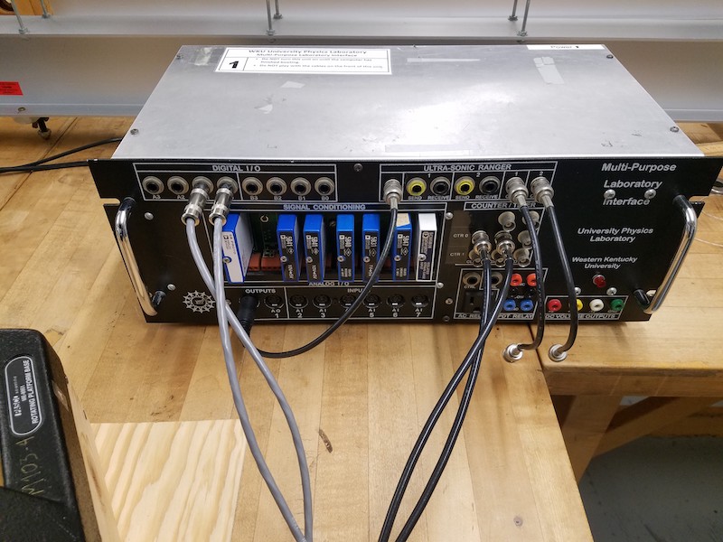 |
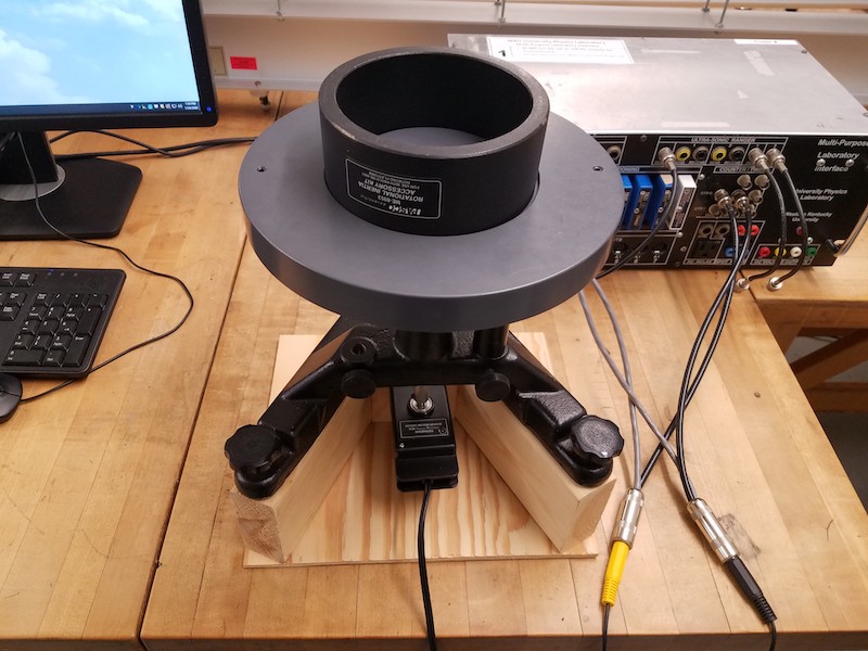
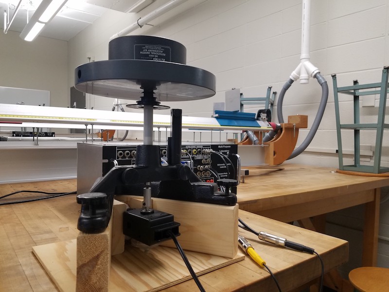
| Figure 1: Rotational Apparatus, Disk + Ring | Figure 2: Encoder for Measuring Angular Position | Figure 3: Encoder Connections to Lab Interface |
The rotational apparatus is pictured in Figure 1 and 2, both of which show the disk sitting on top of the ring. The disk has a small grove just the right size to keep the ring centered on top of it. Careful measurements of the masses and diameters of the disk and ring are given in the table below.
| Mass of Disk | \(M_d=1.4498 \pm 0.0001\) kg |
| Diameter of Disk | \(D_d = 0.2280 \pm 0.0005\) m |
| Mass of Ring | \(M_r = 1.4185 \pm 0.0001\) kg |
| Inside Diameter of Ring | \(D_{ri} = 0.109 \pm 0.001\) m |
| Outside Diameter of Ring | \(D_{ro} = 0.127 \pm 0.001\) m |
Figure 2 shows the encoder attached to the bottom of the apparatus where is it in line with the rotational axis. The encoder outputs a pulse every time the axis rotates thru \(0.25^\circ\), or \(1,440\) pulses per revolution. These pulses are measured by the data acquisition system (depicted in Figure 3) to provide a measurement of the angular position of the system as a function of time. The angular position data is numerically integrated in the Physics Lab Assistant software to obtain the angular velocity.
The system is set into motion by spinning the disk by hand. The data acquisition system begins measuring the angular position and calculating the angular velocity as a function of time. The ring is dropped onto the disk and after a short amount of time when the two objects are spinning together the data acquisition is stopped. An example of a data file is provided below. This file is in a tab-delimited text format and can be loaded directly into Physics Data Assistant. After doing so you should create a graph of angular position as a function of time and a graph of angular velocity as a function of time.
When you plot the angular position as a function of time you will notice it initially increases at what appears to be a constant rate where it was set into spinning motion. If this were a perfectly linear increase then the angular velocity would be constant. However, you will notice in your graph of angular velocity that it decreases very slightly. This is due to the disk slowing down slightly over time due to the small frictional torque that is present in the rotational bearings of the system. The sudden kink in the angular position graph depicts where the ring was dropped onto the disk. The rate of increase of angular position drops dramatically in this interval. You can see this best on the graph of angular velocity versus time. On this graph you should be able to identify clearly the following three regions:
- Before the collision: the angular velocity is slowly decreasing due to friction in the bearings of the apparatus.
- During the collision: the angular velocity is dropping rapidly as the ring slides on the disk until it eventually moves at the same rate as the disk.
- After the collision: the angular velocity once again slowly decreases due to friction in the bearings of the apparatus.
You should be able to place cursors on your graph of angular velocity versus time and read out the angular velocity immediately before and immediately after the collision. With these data, and the appropriate inertia values, you should be able to compute the initial and final angular momentum of the system to see if angular momentum is conserved. In a similar manner you can also compare the initial and final rotational kinetic energy of the system.
Simulation
The following starter code is useful to attempting to model this rotational coupling collision.
#
# E3C - Axial Coupling
#
# Model an axial coupling style collision of a ring dropped onto a rotating disk
#

# Create a disk object centered at the origin.
# Give it a metallic texture so we can see it rotating.
###########################################################################
#                                                                         #
# A - Measure and enter the mass and radius of the disk in the attributes #
#     below and enter the initial anglar velocity of the rotating disk.   #
#                                                                         #
###########################################################################

disk = cylinder(pos=vector(0,0,0), axis=vector(0, 0.015, 0), texture=textures.metal)
disk.radius = 0.113                             # Radius of the disk [m]
disk.mass = 1.443                               # Mass of the disk [kg]
disk.inertia = 0.5*disk.mass*disk.radius**2     # Rotational inertia of the disk [kg m**2]
disk.omega = 10                                 # Initial angular velocity of the disk [rad/s]
disk.L = disk.inertia * disk.omega              # Initial angular momentum of the disk [kg m**2 rad/s]


# Create a ring object and place it centered on and about 5 cm above the disk
###########################################################################
#                                                                         #
# B - Measure and enter the mass and radius of the hoop in the attributes #
#     below.                                                              #
#                                                                         #
###########################################################################
hoop=ring( pos=vec(0,.05,0), axis=vec(0,1,0), texture=textures.rough)
hoop.radius = 0.06                              # Radius of hoop [m]
hoop.size=vector(0.015,hoop.radius*2,hoop.radius*2)
hoop.mass=1.431                                 # Mass of hoop [kg]
hoop.inertia=hoop.mass*hoop.radius**2           # Rotational inertia [kg m**2]
hoop.omega =0                                   # Initial angular velocity [rad/s]
hoop.L = 0                                      # Initial angular momentum [kg m**2 rad/s]

# Create a Angular Velocity vs Time Graph
velocityGraph = graph(title='Angular Velocity vs Time',
    xtitle='Time (s)', ytitle='Angular Velocity (rad/s)',
    fast=False, width=800)
diskVelocity = gcurve(color=color.red, width=2, label='Disk')
hoopVelocity = gcurve(color=color.blue, width=2, label='Hoop')

# Creae an Angular Momentum vs Time Graph
momentumGraph = graph(title='Angular Momentum vs Time',
    xtitle='Time (s)', ytitle='Angular Momentum (kg m**2/s)',
    fast=False, width=800)
diskMomentum = gcurve(color=color.red, width=2, label='Disk')
hoopMomentum = gcurve(color=color.blue, width=2, label='Hoop')
totalMomentum = gcurve(color=color.black, width=2, label='Total')

# Define the axis of rotation vector to be in the y-direction
n = vector(0,1,0)

# Define necessary constants
g = 9.8             # Acceleration due to gravity [N/kg]
dt = 0.002          # Time step [s]
t=0                 # Time counter [s]
droptime = 5.25     # Time when hoop is dropped [sec]
mu = 0.25           # Coefficient of kinetic friction between hoop and ring [estimate]

###########################################################################
#                                                                         #
# C - Define an appropriate value for the frictional torque experienced   #
#     by the rotating disk when it is is spinning freely. This torque is  #
#     due to friction in the bearings of the rotational apparatus.        #
#                                                                         #
#     Estimate a value for this quantity from measurements of the angular #
#     velocity of the disk vs time while freely spinning.                 #
#                                                                         #
###########################################################################
friction_torque = 0                      # Frictional torque [N m]
#
# The contact_torque is the torque on the disk by the hoop while they are
# sliding on each other during the axial coupling collision.  It is due to
# sliding friction between the disk and the hoop.
contact_torque  = -(mu * hoop.mass * g) * hoop.radius

# Run for a set amount of time
while (t < 20):
    rate(2000)

    # We have three distinct time intervals of interest.
    #
    #  1. Before the hoop is dropped (t < droptime) when the disk is spinning
    #     and the hoop is stationary.
    #
    #  2. After the hoop has been dropped onto the disk but before they are
    #     moving together as one unit.  The hoop and disk are slipping relative
    #     to one another.  Here the angular velocity of the hoop will have a
    #     smaller absolute value than that of the disk.
    #
    #  3. After the hoop and the ring are moving together with the same angular
    #     velocity.

    if (t < droptime): # Interval 1

        # D - Enter expression for the net Torque during this time interval
        net_torque = 0

        # E - Update the angular momentum of the disk
        disk.L = 0

        # F - Update the angular velocity of the disk
        disk.omega = 0

        # Update the angular position of the disk
        disk.rotate(angle=disk.omega*dt, axis=n)

    else if(abs(hoop.omega) < abs(disk.omega)): # Interval 2

        # Drop the hoop onto the disk by lowering it's vertial position.
        hoop.pos.y = 0.015

        # G - Enter an expression for the net torque ON THE DISK
        net_torque = 0

        # Update angular momentum, angular velocity and angular position of the disk
        disk.L = disk.L + net_torque * dt
        disk.omega = disk.L/disk.inertia
        disk.rotate(angle=disk.omega*dt, axis=n)

        # H - Enter an expression for the net torque ON THE HOOP
        net_torque = 0

        # Update angular momentum, angular velocity and angular position of the hoop
        hoop.L = hoop.L + net_torque * dt
        hoop.omega = hoop.L/hoop.inertia
        hoop.rotate(angle=hoop.omega*dt, axis=n)

    else:   # Interval 3 - Both objects move together

        # I - Enter an expression for the net torque on the system (disk + hoop)
        net_torque = 0

        disk.L =disk.L+ net_torque * disk.inertia/(disk.inertia+hoop.inertia) * dt
        disk.omega = disk.L / disk.inertia
        disk.rotate(angle=disk.omega*dt, axis=n)

        hoop.L = hoop.L+ net_torque * hoop.inertia/(disk.inertia+hoop.inertia) * dt
        hoop.omega = hoop.L/hoop.inertia
        hoop.rotate(angle=hoop.omega*dt, axis=n)

    # Increment the time counter
    t=t+dt

    # Plot the angular velocities
    diskVelocity.plot(t, disk.omega)
    hoopVelocity.plot(t, hoop.omega)

    # Plot the angular momenta
    diskMomentum.plot(t, disk.L)
    hoopMomentum.plot(t, hoop.L)
    totalMomentum.plot(t, disk.L+hoop.L)

