Friday, November 15, 2019
The WKU Volleyball team is presently 27-1 on the season and 13-0 in C-USA conference play. On Saturday, November 16, 2019 at noon the team will play its final regular season game against UAB in Diddle Arena. This will be Senior Day where two players, Sophia Cerino (#23) and Emma Kowalkowski (#3), will be honored before the match.
Hilltopper Nation, you were absolutely incredible tonight!
We CAN'T WAIT to see you in Diddle on Saturday at 12pm CST, as @WKUVolleyball tries to win the @ConferenceUSA regular-season title outright! #GoTops pic.twitter.com/C4tQFretCi
— WKU (@wku) November 15, 2019
Sophia is a right-side hitter which means you’ll find her playing on the front line attacking the net looking to score by spiking the ball across the net as well as protecting the net by attempting to block the opposing team. She is the top server in the country, leading the NCAA in aces per set and total aces.
Emma is a defensive specialist which means she plays on the back line and focuses on making the first play on the ball and making a good pass to the setter.
Interestingly, Sophia and Emma share the same spot in the rotation. You’ll see them substitute for each other as the team rotates with Sophia playing the front line spots and Emma the back line spots in the rotation.
Tonight @sophiacerino23 set the @WKUVolleyball single-season record for service aces with 69 after recording 6 in the Lady Tops win over Louisiana Tech.
Except, #SophiACErino didn't even know she had a chance to break the record ? #GoTops pic.twitter.com/RBxNC0Adoc
— Matt Foster WNKY (@MattFosterWNKY) November 15, 2019
I thought it would be interesting to honor the hard-work that these student-athletes have put in this year and to learn a little bit of new physics at the same time.
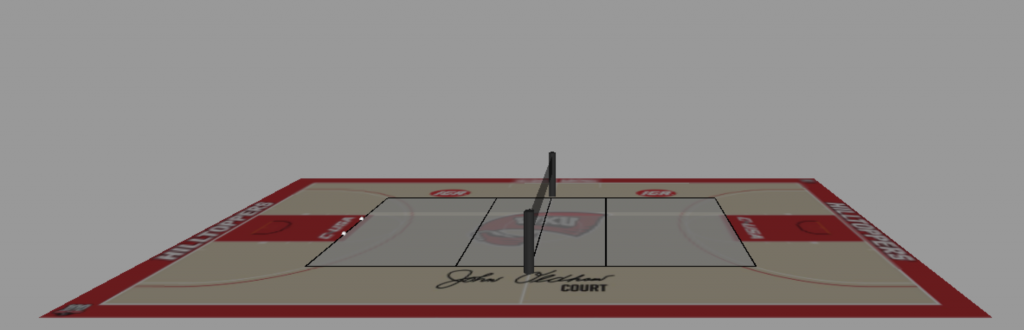
There is some starter VPython code at the bottom of this post that draws a scene representing the volleyball court on the Diddle Arena floor like shown here. There are several comments in the code that identify the coordinate system used and the dimensions of the court.
Your tasks are to:
- Go to the match on Saturday and study the serves of the senior players, Cerino and Kowalkowski. If you get there before the match you’ll have a chance to see many serves during warm ups. You will want to be able to make informed estimates of the initial position and the initial velocity (both linear velocity and angular velocity) as it leaves each of these player’s hands. Notice that players tend to serve from a favorite spot on the floor and they will generally will also warm up from these same locations. Add comments in your code that justify any assumptions and estimates that you make.
Feel free to stop by and say hi before the game. I sit on the first row behind the rail at mid-court in section 105.
- Add commands to the starter code below that will set the parameters
.mfor the mass of the ball,.posfor the initial position of the ball,.vfor the initial velocity of the ball, and.pfor the initial momentum of the ball. - Inside a loop, model the motion of the ball from the moment it leaves the player’s hand after the serve until the moment it hits the floor on the opposite side of the net. Make the ball leave a trail of dots so that the ball’s motion is easily shown on the scene. You will need to compute the net force on the ball, update the ball’s momentum using the momentum principle, and finally update the ball’s position. Do this for the two balls provided in the starter code. One should match the characteristics of Sophia’s serve and one should match Emma’s serve. These will have different initial conditions. Describe how you chose these values in the comments.
- Create graphs showing the trajectories of the balls. Graphs looking from above showing z vs x or and from the side showing y vs x would be interesting.
Some Background
You should obviously include the gravitational force on the ball when computing the net force. In addition, you should include air resistance. As we have discussed previously, an appropriate model for the air resistance would be the following expression where the force is a quadratic function of the ball’s speed and directed opposite to its velocity:
$$\vec{F}_\textrm{air} = -\frac{1}{2}C \rho A v^2 \hat{v}$$
Make an estimate for the bluntness coefficient of the ball \(C\) and the cross-sectional area \(A\) of the ball and specify an appropriate value for the density of air \(\rho\) in kg/m\(^3\).
In addition, you will want to include the Magnus force, which takes into account the effects of the ball’s spin on its motion. This is a new force for us and is the primary reason why the assignment is extra credit. This force can be written as
$$\vec{F}_M = (1/2) C_L \rho A v^2 \hat{\omega} \times \hat{v}$$
where \(C_L\) is a lift coefficient that depends on the spin rate, and \(\vec{\omega}\) is the angular velocity of the volleyball. For our purposes, you can assume that the angular velocity of the ball will remain constant throughout the flight. You are going to have to make some estimates and do some research to obtain a reasonable value for \(C_L\) for each server. You will need to estimate a value for the direction of the angular velocity \(\hat{\omega}\). Use the right-hand rule as we showed in class to help you determine this direction. Notice that direction of the Magnus force is perpendicular to the velocity while the drag force is opposite the velocity.

Assignment Submission Rules
- You may work alone or as a team in a group of up to three students. However, if you work in a group, your code MUST include a short description of how different members of the group contributed to building the model. Add this discussion at the top of the program using comments.
- Collaboration between groups is allowed and encouraged but each group submission is expected to be unique!. Sharing of ideas is good, sharing your final code is not.
- This will be an extra-credit assignment that will add to your VPython portion of your grade. It will be worth a total of 50 possible points.
- This assignment will be due on Tuesday, November 26.
- It is better to submit a link to a program that works with some aspects left out rather than trying to add a feature and having a non-working program. In other words, if you can’t get the Magnus force to work, just leave it out. Partial credit will be given.
- As usual submit a plain text file that contains a list of your group members and a link to your working code on Gradescope. Be sure to follow directions for submitting a group assignment on Gradescope.
Starter Code
# Fall 2019 Extra Credit Program
#  WKU Volleyball Senior Day

# Use a box object to model the Diddle Arena floor.
#
# The size of regulation basketball floor is 94 ft x 50 ft (28.65 m x 15.24 m).
#   https://https://www.recunlimited.com/blog/diagrams-basketball-courts/
#
# The floor at Diddle Arena has borders on the sides and ends that we will
# approximate as 3 ft.  Adding these extra borders makes
# for a dimension of 104 ft x 56 ft (31.70 m x 17.07 m).
#
# We will place the origin at the enter of the court and will use our standard
# coordinate system with x and z horizontal and y vertical.  The x-axis
# will be along the long dimension and the z-axis will be along midcourt.

floor = box(pos=vector(0,-0.01,0), length=31.70, width=17.07, height=0.01, texture="https://i.imgur.com/ZH6eZFl.png")

# Raise the camera position a few meters so that we are not looking at the floor
# edge on and move it to the side a bit to the net is more easily visible.

scene.camera.pos = scene.camera.pos + vector(3, 10, 0)

# Adjust the scene size and background color to make the animation more visible
scene.width = 1400
scene.height = 800
scene.background = vector(0.6, 0.6, 0.6)

# Use another box to model the volleyball court playing area.
#
# An NCAA Volleyball court is 18m x 9m.
#   http://www.ncaapublications.com/productdownloads/VBR19.pdf [see Rule 1]
#
# We'll draw this box just slightly above the Diddle Arena floor and make it
# opaque so we can still see the floor.

court = box(pos=vector(0, 0.01, 0), length=18, width=9, height=0.01, color=color.white, opacity=0.5)

# Draw the lines on the volleyball court and the supports for the net.
lw = 0.05           # Line width = 2 inches = 5 cm
lh = 0.02
lc = color.black    # Line color
left_end  = box(pos=vector(-9, 0.02, 0), length=lw, width=9, height=lh, color=lc)
left_attack  = box(pos=vector(-3, 0.02, 0), length=lw, width=9, height=lh, color=lc)
center    = box(pos=vector(0, 0.02, 0), length=lw, width=9, height=lh, color=lc)
left_attack  = box(pos=vector(+3, 0.02, 0), length=lw, width=9, height=lh, color=lc)
right_end = box(pos=vector(+9, 0.02, 0), length=lw, width=9, height=lh, color=lc)
near_sideline = box(pos=vector(0, 0.02, -4.5), length=18, width=lw, height=lh, color=lc)
far_sideline = box(pos=vector(0, 0.02, +4.5), length=18, width=lw, height=lh, color=lc)

sc = vector(0.2, 0.2, 0.2)
near_support = cylinder(pos=vector(0, 0, -5), axis=vector(0,1,0), length=2.4, radius=0.2, color=sc)
far_support  = cylinder(pos=vector(0, 0, +5), axis=vector(0,1,0), length=2.4, radius=0.2, color=sc)

# Finally, another box will be used to model the net.
#
# The height of the top of the women's volleball net is 7 ft 4.125 inches (2.24m)
# above the floor. The net itself is 1m tall and 9.5 m long.
#   http://www.ncaapublications.com/productdownloads/VBR19.pdf [see Rule 2]
#
# Thus, in our coordinate system, the center of the net will be at a vector position of
#    <0, 2.24 - 0.5, 0> m = <0, 1.74, 0> m.

net = box(pos=vector(0, 1.74, 0), length=0.01, width= 9.5, height=1.0, color=color.black, opacity=0.3)

# Use a sphere object to model the volleyballs.
#
# The NCAA regulations specify a requirement for the ball's circumference.  It must be
# between 65 cm and 67 cm.
#   http://www.ncaapublications.com/productdownloads/VBR19.pdf [see Rule 3]
#
# So we'll use 66 cm which will correspond to a radius of
#  66 cm / (2 * pi) = 10.5 cm = 0.105 m.
#
# I considered adding a texture to the ball to make it look like a volleyball,
# but on this scale it would be difficult to see and perhaps not worth the effort.
#

# Create two balls, one for Sophia (ball1) and one for Emma (ball2).

ball1 = sphere(radius=0.105, color=color.white)
ball2 = sphere(radius=0.105, color=color.white)

# Add attributes for the balls.
#
# I will set the balls down on the floor near the center of the end line of the
# volleyball court.

ball1.pos = vector(-9, 0.05, -1)
ball2.pos = vector(-9, 0.05, +1)

# You will want to estimate appropriate values for the
#   * initial positions (.pos) for each ball as they leave the servers' hands
#   * the masses (.m),
#   * initial linear velocities (.v),
#   * initial linear momenta (.p), and
